Файл:AdaptiveBeamForming.png
Перейти к навигации
Перейти к поиску

Размер этого предпросмотра: 800 × 405 пкс. Другие разрешения: 320 × 162 пкс | 640 × 324 пкс | 1291 × 653 пкс.
Исходный файл (1291 × 653 пкс, размер файла: 78 КБ, MIME-тип: image/png)
Этот файл находится на Викискладе. Сведения о нём показаны ниже.
Викисклад — централизованное хранилище для свободных файлов, используемых в проектах Викимедиа.
|
Краткое описание
| Описание |
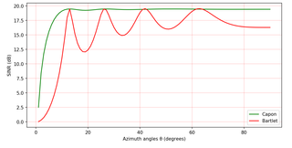
English: An example of Adaptive Beamforming (source code).
Русский: Пример адаптивного диаграммообразования (исходный код). |
| Дата | |
| Источник | Собственная работа |
| Автор | Kirlf |
| PNG‑разработка | Это plot было создано с помощью Matplotlib |
| Исходный код | Python code"""
Developed by Vladimir Fadeev
(https://github.com/kirlf)
Kazan, 2017 / 2020
Python 3.7
"""
import numpy as np
import matplotlib.pyplot as plt
"""
Received signal model:
X = A*S + N
where
A = [a(theta_1) a(theta_2) ... a(theta_d)]
is the matrix of steering vectors
(dimension is M x d,
M is the number of sensors,
d is the number of signal sources),
A steering vector represents the set of phase delays
a plane wave experiences, evaluated at a set of array elements (antennas).
The phases are specified with respect to an arbitrary origin.
theta is Direction of Arrival (DoA),
S = 1/sqrt(2) * (X + iY)
is the transmit (modulation) symbols matrix
(dimension is d x T,
T is the number of snapshots)
(X + iY) is the complex values of the signal envelope,
N = sqrt(N0/2)*(G1 + jG2)
is additive noise matrix (AWGN)
(dimension is M x T),
N0 is the noise spectral density,
G1 and G2 are the random Gussian distributed values.
"""
M = 9 # number of antenna elements (sensors)
""" Correlation matrix of the information symbols:
Rss = S*S^H = I_d (try with QPSK, for example) """
Rss = np.eye((2))
""" Correlation matrix of additive noise:
Rnn = N*N^H = sigma_N^2 * I_M),
where sigma_N^2 is the noise variance (power) """
Rnn = 0.1*np.eye((M)) #
""" Let us consider 2 sources of the signals """
theta_1 = 0*(np.pi/180)
theta_2 = 50*(np.pi/180)
""" Spatial frequency (some equivalent of a DoA):
mu = (2*pi / lambda ) * delta * sin(theta)
where
delta is the antenna spacing
(distance between antenna elements), and
lambda is the electromagnetic wave length.
Let us (delta = lambda / 2) then:
"""
mu_1 = np.pi*np.sin(theta_1)
mu_2 = np.pi*np.sin(theta_2)
""" Steering vectors """
a_1 = np.exp(1j*mu_1*np.arange(M))
a_2 = np.exp(1j*mu_2*np.arange(M))
A = (np.array([a_1, a_2])).T
"""
Correlation matrix of the received signals
R_xx = X*X^H = A*R_ss*A^H + R_nn
"""
R = A @ Rss @ np.conj(A).T + Rnn
""" Let us theta_1 is the signal, and theta_2 is the interferer """
g = np.array([1, 0]) # the first DoA is "switched on", the second DoA is "switched off".
def calc_w_capon(A_i):
""" Capon's method (MVDR)
w_Capon = R^(-1) * A * (A^H * R^(-1) * A)^(-1) * g """
w = (np.linalg.inv(R) @ A_i @
np.linalg.inv( np.conj(A_i).T @ np.linalg.inv(R) @ A_i ) @ g).T
return w
def calc_power(w, a):
""" P(theta) = abs(w_(opt)^H * a(theta))^2 """
P = (np.abs( (np.conj(w).T @ a) )**2).item()
return P
""" Bartlett's method (сonventional beamforming)
w_Bart = a_1 / M """
w_bart = (a_1 / M).reshape((M,1))
""" Simulation loop.
Main idea:
1) We have the Rxx matrix from the receiver.
2) We know the DoA of the information signal and
DoA of the interference (e.g., based on frequency estimation methods)
3) We should calculate optimal weight vector which will suppress interference.
4) This should make SINR (Signal to Interference + Noise Ratio) better.
5) Interference DoA can changes, but estimated Rxx should be the same!
"""
sinr_thetas = np.arange(1, 91)*(np.pi/180) # degrees (from 1 to 90) -> radians
SINR_Capon = np.empty(len(sinr_thetas), dtype = complex)
SINR_Bart = np.empty(len(sinr_thetas), dtype = complex)
for idx, theta_i in enumerate(sinr_thetas):
""" Let's try to simulate changing of the interference picture!
For this redefine DoA of intereference. """
mu_2 = np.pi*np.sin(theta_i)
a_2 = np.exp(1j*mu_2*np.arange(M))
A_sinr = (np.array([a_1, a_2])).T
""" Capon's (MVDR) method: """
w_capon = calc_w_capon(A_sinr)
signal_capon = calc_power(w_capon, a_1)
interf_capon = calc_power(w_capon, a_2)
""" P_noise = w^H * Rnn * w """
noise_capon = (np.conj(w_capon).T @ Rnn @ w_capon).item()
""" SINR - Signal to Interference + Noise Ratio """
SINR_Capon[idx] = signal_capon / (interf_capon + noise_capon)
""" Bartlett's method
(uses the same weight vector for every cases - not adaptive): """
signal_bart = calc_power(w_bart, a_1)
interf_bart = calc_power(w_bart, a_2)
noise_bart = (np.conj(w_bart).T @ Rnn @ w_bart).item()
SINR_Bart[idx] = signal_bart / (interf_bart + noise_bart)
"""
Capon's method is more stable,
Bartlett's method cannot well mitigate changed interference.
"""
plt.subplots(figsize=(10, 5), dpi=150)
plt.plot(sinr_thetas*(180/np.pi), 10*np.log10(np.real(SINR_Capon)), color='green', label='Capon')
plt.plot(sinr_thetas*(180/np.pi), 10*np.log10(np.real(SINR_Bart)), color='red', label='Bartlett')
plt.grid(color='r', linestyle='-', linewidth=0.2)
plt.xlabel('Azimuth angles θ (degrees)')
plt.ylabel('SINR (dB)')
plt.legend()
plt.show()
""" References
1. Haykin, Simon, and KJ Ray Liu.
Handbook on array processing and sensor networks.
Vol. 63. John Wiley & Sons, 2010. pp. 102-107
2. Haykin, Simon S.
Adaptive filter theory.
Pearson Education India, 2008. pp. 422-427
3. Richmond, Christ D.
"Capon algorithm mean-squared error threshold
SNR prediction and probability of resolution." IEEE
"""
|
Лицензирование
Я, владелец авторских прав на это произведение, добровольно публикую его на условиях следующей лицензии:
Этот файл доступен по лицензии Creative Commons Attribution-Share Alike 4.0 International
- Вы можете свободно:
- делиться произведением – копировать, распространять и передавать данное произведение
- создавать производные – переделывать данное произведение
- При соблюдении следующих условий:
- атрибуция – Вы должны указать авторство, предоставить ссылку на лицензию и указать, внёс ли автор какие-либо изменения. Это можно сделать любым разумным способом, но не создавая впечатление, что лицензиат поддерживает вас или использование вами данного произведения.
- распространение на тех же условиях – Если вы изменяете, преобразуете или создаёте иное произведение на основе данного, то обязаны использовать лицензию исходного произведения или лицензию, совместимую с исходной.
История файла
Нажмите на дату/время, чтобы посмотреть файл, который был загружен в тот момент.
| Дата/время | Миниатюра | Размеры | Участник | Примечание | |
|---|---|---|---|---|---|
| текущий | 05:37, 18 февраля 2019 | | 1291 × 653 (78 КБ) | Kirlf | User created page with UploadWizard |
Использование файла
Следующая страница использует этот файл: