Файл:Lemniscates5.png

Исходный файл (1000 × 1000 пкс, размер файла: 73 КБ, MIME-тип: image/png)
Этот файл находится на Викискладе. Сведения о нём показаны ниже.
Викисклад — централизованное хранилище для свободных файлов, используемых в проектах Викимедиа.
|

|
Этот график желательно воссоздать или аккуратно преобразовать в векторный формат SVG. Это даёт несколько преимуществ, прочитать о которых подробнее вы можете на странице Commons:Media for cleanup. Если вам уже сейчас доступна векторная версия данного изображения, загрузите её, пожалуйста, а затем замените этот шаблон на следующий: {{Vector version available|Имя загруженного файла.svg}}.
|
Краткое описание
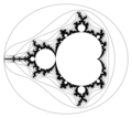
| Описание | 6 lemniscates of Mandelbrot set. Computed using implicit equations. |
| Источник | self-made with help of many people, using free CAS Maxima, Gnuplot and implicit_plot package (by Andrej Vodopivec) |
| Автор | Adam majewski |
| Другие версии | lemniscates for Julia set |
Compare with
-
 DEM and sobel
 -
 LCM/J; ER=1000
 -
 LCM/J but better algorithm, ER = 2
 -
 LSM/J B&W; ER = 1000
 -
 LSM/J colour ( probably made with Fractint ); ER = 2


See also:
Long description
" instead of iterating a point through a nice fractal-generating function until it exits the containing circle, I'm starting with the containing circle's function (2cos(t),2sin(t)) and iterating that circle function through the inverse of the fractal-generating function." Axis Angels[1]
Few lemniscates of Mandelbrot set[2]. They are boundaries of Level Sets of escape time ( LSM/M [3]).
They are in parameter plane (c-plane, complex plane ).
Definition :

where
is Escape Radius, bailout value, radius of circle which is used to measure if orbit of is bounded; it is integer number


are complex numbers (points of 2-D planes )

is point of dynamical plane ( z-plane)

is point of parameter plane ( c-plane)


One can compute first few iterations :


and so on .
Then :


...
is a circle,

is an Cassini oval,


These curves tend to boundary of Mandelbrot set as n goes to infinity.
If ER < 2 they are inside Mandelbrot set[6].
If ER = 2 curves meet together ( have common point) c = −2. Thus they can't be equipotential lines.
If ER ≥ 2 they are outside of Mandelbrot set. They can also be drawn using Level Curves Method.
If ER >> 2 they aproximate equipotential lines ( level curves of real potential , see CPM/M ).
Maxima source code
 /* based on the code by Jaime Villate */
 load(implicit_plot); /* package by Andrej Vodopivec */

 c: x+%i*y;

 ER:2; /* Escape Radius = bailout value it should be >=2 */

 f[n](c) := if n=1 then c else (f[n-1](c)^2 + c);

 ip_grid:[100,100];  /* sets the grid for the first sampling in implicit plots. Default value: [50, 50] */
 ip_grid_in:[15,15]; /* sets the grid for the second sampling in implicit plots. Default value: [5, 5] */

 my_preamble: "set zeroaxis; set title 'Boundaries of level sets of escape time of Mandelbrot set'; set xlabel 'Re(c)';  set ylabel 'Im(c)'";

 implicit_plot(makelist(abs(ev(f[n](c)))=ER,n,1,6), [x,-2.5,2.5],[y,-2.5,2.5],[gnuplot_preamble, my_preamble],
 [gnuplot_term,"png   size  1000,1000"],[gnuplot_out_file, "lemniscates6.png"]);
For curves 1-5 it works, but for curve number 6 this program fails( also Mathematica program[7]), because of floating point error.
One have to change the method of computing lemniscates . Here is the code and explanation by Andrej Vodopivec" "You can trick implicit_plot to do computations in higher precision. Implicit_draw will draw the boundary of the region where the function has negative value. You can define a function f6 which computes the sign of f[6] using bigfloats and then plot f6."
/* based on the code by Jaime Villate and Andrej Vodopivec*/
c: x+%i*y;
ER:2;
f[n](c) := if n=1 then c else (f[n-1](c)^2 + c);
F(x,y):=block([x:bfloat(x), y:bfloat(y)],if abs((f[6](c)))>ER then 1 else -1);
fpprec:32;
load(implicit_plot); /* package by Andrej Vodopivec */
ip_grid:[100,100];
ip_grid_in:[15,15];
implicit_plot(append(makelist(abs(ev(f[n](c)))=ER,n,1,5), ['(F(x,y))]),[x,-2.5,2.5],[y,-2.5,2.5]);
Questions
- What is mathemathical description of these curves ?
Rerferences
- ↑ You tube video
- ↑ lemniscates at Mandelbrot Set Glossary and Encyclopedia, by Robert Munafo
- ↑ LSM/M
- ↑ Weisstein, Eric W. "Pear Curve." From MathWorld--A Wolfram Web Resource. http://mathworld.wolfram.com/PearCurve.html
- ↑ Mandelbrot lemniscate at 2DCurves by Jan Wassenaar
- ↑ Polynomial_lemniscate
- ↑ | Weisstein, Eric W. "Mandelbrot Set Lemniscate." From MathWorld--A Wolfram Web Resource.
Лицензирование

|
Разрешается копировать, распространять и/или изменять этот документ в соответствии с условиями GNU Free Documentation License версии 1.2 или более поздней, опубликованной Фондом свободного программного обеспечения, без неизменяемых разделов, без текстов, помещаемых на первой и последней обложке. Копия лицензии включена в раздел, озаглавленный GNU Free Documentation License. |
- Вы можете свободно:
- делиться произведением – копировать, распространять и передавать данное произведение
- создавать производные – переделывать данное произведение
- При соблюдении следующих условий:
- атрибуция – Вы должны указать авторство, предоставить ссылку на лицензию и указать, внёс ли автор какие-либо изменения. Это можно сделать любым разумным способом, но не создавая впечатление, что лицензиат поддерживает вас или использование вами данного произведения.
- распространение на тех же условиях – Если вы изменяете, преобразуете или создаёте иное произведение на основе данного, то обязаны использовать лицензию исходного произведения или лицензию, совместимую с исходной.
История файла
Нажмите на дату/время, чтобы посмотреть файл, который был загружен в тот момент.
| Дата/время | Миниатюра | Размеры | Участник | Примечание | |
|---|---|---|---|---|---|
| текущий | 19:42, 11 января 2009 | | 1000 × 1000 (73 КБ) | Geek3 | smooth and precise plotcurve |
| 10:22, 18 марта 2008 |  | 1000 × 1000 (17 КБ) | Soul windsurfer | added 6 lemniscate | |
| 08:15, 16 марта 2008 |  | 1000 × 1000 (15 КБ) | Soul windsurfer | {{Information |Description= |Source=self-made |Date= |Author= Adam majewski |Permission= |other_versions= }} |
Использование файла
Нет страниц, использующих этот файл.
Глобальное использование файла
Данный файл используется в следующих вики:
- Использование в ca.wikipedia.org
- Использование в en.wikibooks.org
- Использование в sl.wikipedia.org